PlantSimEngine.jlBuild plant simulations from connected process models
Combine models of growth and plant–environment interactions in Julia, from crop canopies to individual plants and organs.
Combine models of growth and plant–environment interactions in Julia, from crop canopies to individual plants and organs.

PlantSimEngine connects and runs models of plant processes such as light interception, photosynthesis and growth. You choose the equations, using existing model packages or writing your own. PlantSimEngine manages their connections, execution order, time steps and simulation outputs in Julia.
You can represent a whole crop canopy, individual plants, or their organs. You choose the level of detail; 3D geometry is optional. Small, testable models and clear reports on their connections also support AI-assisted model development.
For scientific equations, explore packages such as PlantBiophysics.jl, for plant biophysical processes, and XPalm, for oil-palm growth. Their documentation describes the models, assumptions and supported package versions.
PlantSimEngine helps bridge the gap between crop and functional–structural modelling by letting you develop a common core of process models and choose the level of structural detail your question needs. Represent a canopy as a whole, describe individual organs, or include their positions in 3D. Reuse the shared models and adapt the processes and connections that depend on that detail.
XPalm illustrates this approach: its core growth and development models can run with or without a 3D representation of the palm. This provides a foundation for investigating questions about spatial differences in light or local carbon allocation, by adding the appropriate models while retaining the shared core.
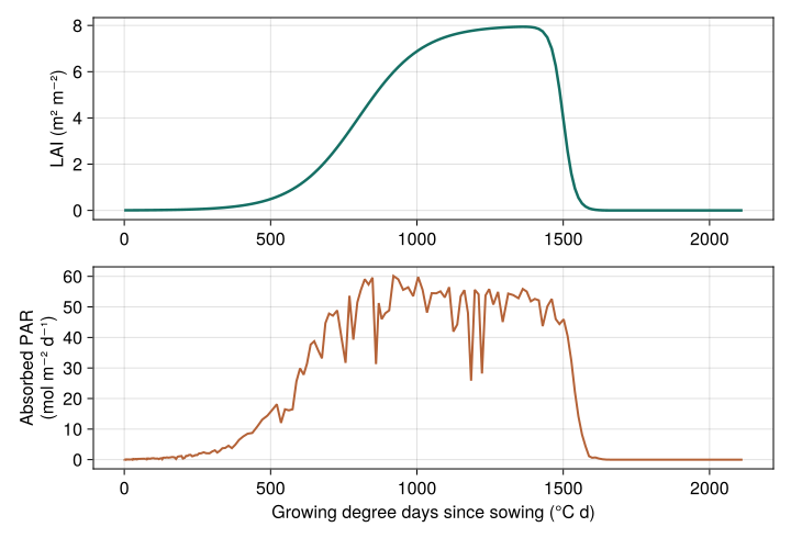
These examples illustrate two levels of detail: a whole crop canopy and a plant described by individual organs.
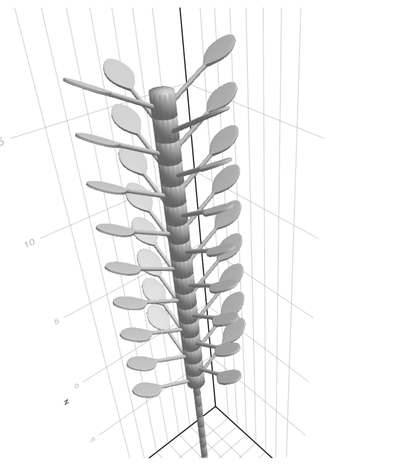
For plant–environment interactions, the MAESPA-style example combines two species, leaf exchanges, soil water and daily growth. It is an advanced teaching example of coupling these processes, rather than a validated reproduction of MAESPA.
What happens if carbon gain stops increasing in proportion to absorbed light? Here, the same small simulation is run with a linear response and then a saturating response. Only the carbon-gain model changes. Both models simulate the same process, so we can just replace one by another, and PlantSimEngine handles the rest: how, where and when the model is called, relative to other models, objects (organs/plants/scene), and simulation rate.
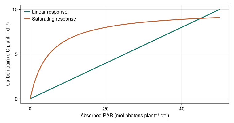
The models come from the examples supplied for model authors and AI agents. Follow the model replacement guide to try alternatives and check whether their inputs require different connections.
Keep equations separate from the scenario. Write a process model once, then choose which plants or organs use it, its parameters and its connections. Reuse models across several plants.
Combine different time steps. Connect hourly exchanges and daily growth, stating when values should be accumulated, averaged or held between updates. Connect hourly and daily models.
Follow changes in plant structure. Add or remove organs during a simulation and let PlantSimEngine update the affected model connections. Model a changing structure.
Inspect what is connected. Find the source of an input, inspect the execution order and diagnose missing or ambiguous connections. Explore a model graph.
Control interactions that need iteration. For example, a canopy solver can repeatedly call leaf models until an energy balance converges, then record the accepted result. Control iterative calculations.
Run repeated simulations efficiently. PlantSimEngine prepares model connections before the time loop and reuses them during execution. This avoids resolving those connections again at every time step, including when models run on many organs. Read about the design and performance of PlantSimEngine.
An AI coding agent is software that can read and edit code and run tests with your development tools. Think OpenAI's ChatGPT App (formerly Codex), Anthropic's Claude Code, SpaceXAI's Grok Bot, or Mistral's Vibe. PlantSimEngine is designed to support this way of working, so you can just make new models, compare hypothesis, make model calibration or anything you'd like with just a prompt, such as:
Replace the radiation-use efficiency approach I'm using at the moment in my model by the FvCB, Medlyn and Monteith models from PlantBiophysics. Apply them at an hourly rate first, then at half-hourly, and compare the impact on yield of the three approaches. Report the results through dynamic graphs and statistics.
For optimum results, ask your agent to install the agent skill. It'll give your agent concrete information to implement, inspect and check models. Then, it will have access to every detail of the simulation, so you'll be able to ask it complex prompts such as:
Yield simulation is too low compared to data in 2025 and 2026, can you check why?
| Your next step | What you will do |
|---|---|
| Couple existing models | Start with three teaching models, supply weather, run a simulation and read its results. |
| Write a process model | Implement an equation, declare its inputs and outputs, test it and use it in a simulation. |
| Understand how the pieces fit together | Learn the few ideas shared by both workflows, before reading detailed configuration. |
The examples introduce Julia as it is needed. If you are new to the language, start with installation and Julia basics.
The canopy example above connects three existing models: temperature drives thermal time, thermal time drives LAI, and LAI and radiation determine absorbed photosynthetically active radiation (PAR).
First follow the installation instructions to get the package version used by this manual and the tutorial dependencies.
Read the weather supplied with PlantSimEngine. This file stores daily radiation totals in MJ m⁻² d⁻¹; the three conversions below give the mean fluxes in W m⁻² required by the light-interception model.
using PlantSimEngine, PlantMeteo, Dates, DataFrames
using PlantSimEngine.Examples

meteo_day = read_weather(
    joinpath(pkgdir(PlantSimEngine), "examples/meteo_day.csv"),
    :Ri_SW_f => (x -> x .* 1e6 ./ 86_400) => :Ri_SW_f,
    :Ri_PAR_f => (x -> x .* 1e6 ./ 86_400) => :Ri_PAR_f,
    :Ri_NIR_f => (x -> x .* 1e6 ./ 86_400) => :Ri_NIR_f;
    duration=Dates.Day,
)
Choose the models and run the full weather year:
model = CompositeModel(
    ToyDegreeDaysCumulModel(),
    ToyLAIModel(),
    Beer(0.6);
    environment=meteo_day,
)

simulation = run!(model; steps=length(meteo_day), outputs=:all)
results = collect_outputs(simulation; sink=DataFrame)
The thermal-time model supplies the LAI model, which supplies the light model. PlantSimEngine connects them using their matching input and output names. The result table contains their outputs over time. The step-by-step tutorial explains these connections and shows how to continue a simulation; the plotting guide explains how to display results.
PlantSimEngine provides the simulation tools. Model packages provide equations, parameters and their scientific validation. Examples of packages using PlantSimEngine include:
PlantBiophysics.jl, for plant biophysical processes such as photosynthesis, stomatal conductance and energy balance.
XPalm, for oil-palm growth and development.
Their documentation describes the models available, their assumptions and supported package versions. To choose an approach, read Why PlantSimEngine?. For a published application and its validation, see the PlantBiophysics paper.
PlantSimEngine is open source under the MIT license. For questions or feedback, open an issue or join the Virtual Plant Lab discussion.



