PlantSimEngine
![]()
![]()
![]()
![]()

Overview
PlantSimEngine is a comprehensive package for simulating and modelling plants, soil and atmosphere. It provides tools to prototype, evaluate, test, and deploy plant/crop models at any scale. At its core, PlantSimEngine is designed with a strong emphasis on performance and efficiency.
The package defines a framework for declaring processes and implementing associated models for their simulation.
It focuses on key aspects of simulation and modeling such as:
- Easy definition of new processes, such as light interception, photosynthesis, growth, soil water transfer...
- Fast, interactive prototyping of models, with constraints to help users avoid errors, but sensible defaults to avoid over-complicating the model writing process
- No hassle, the package manages automatically input and output variables, time-steps, objects, soft and hard coupling of models with a dependency graph
- Switch between models without changing any code, with a simple syntax to define the model to use for a given process
- Reduce the degrees of freedom by fixing variables, passing measurements, or using a simpler model for a given process
- 🚀(very) fast computation 🚀, think of 100th of nanoseconds for one model, two coupled models (see this benchmark script), or the full energy balance of a leaf using PlantBiophysics.jl that uses PlantSimEngine
- Out of the box Sequential, Parallel (Multi-threaded) or Distributed (Multi-Process) computations over objects, time-steps and independent processes (thanks to Floops.jl)
- Easily scalable, with methods for computing over objects, time-steps and even Multi-Scale Tree Graphs
- Composable, allowing the use of any types as inputs such as Unitful to propagate units, or MonteCarloMeasurements.jl to propagate measurement error
Installation
To install the package, enter the Julia package manager mode by pressing ] in the REPL, and execute the following command:
add PlantSimEngineTo use the package, execute this command from the Julia REPL:
using PlantSimEngineExample usage
The package is designed to be easy to use, and to help users avoid errors when implementing, coupling and simulating models.
Simple example
Here's a simple example of a model that simulates the growth of a plant, using a simple exponential growth model:
# ] add PlantSimEngine
using PlantSimEngine

# Import the examples defined in the `Examples` sub-module
using PlantSimEngine.Examples

# Define the model:
model = ModelList(
    ToyLAIModel(),
    status=(TT_cu=1.0:2000.0,), # Pass the cumulated degree-days as input to the model
)

run!(model) # run the model

status(model) # extract the status, i.e. the output of the model
TimeStepTable{Status{(:TT_cu, :LAI), Tuple{...}(2000 x 2):
╭─────┬─────────┬────────────╮
│ Row │ TT_cu │ LAI │
│ │ Float64 │ Float64 │
├─────┼─────────┼────────────┤
│ 1 │ 1.0 │ 0.00560052 │
│ 2 │ 2.0 │ 0.00565163 │
│ 3 │ 3.0 │ 0.00570321 │
│ 4 │ 4.0 │ 0.00575526 │
│ 5 │ 5.0 │ 0.00580778 │
│ 6 │ 6.0 │ 0.00586078 │
│ 7 │ 7.0 │ 0.00591426 │
│ 8 │ 8.0 │ 0.00596823 │
│ 9 │ 9.0 │ 0.00602269 │
│ 10 │ 10.0 │ 0.00607765 │
│ 11 │ 11.0 │ 0.00613311 │
│ 12 │ 12.0 │ 0.00618908 │
│ 13 │ 13.0 │ 0.00624556 │
│ 14 │ 14.0 │ 0.00630255 │
│ 15 │ 15.0 │ 0.00636006 │
│ ⋮ │ ⋮ │ ⋮ │
╰─────┴─────────┴────────────╯
1985 rows omitted
Note The
ToyLAIModelis available from the examples folder, and is a simple exponential growth model. It is used here for the sake of simplicity, but you can use any model you want, as long as it followsPlantSimEngineinterface.
Of course you can plot the outputs quite easily:
# ] add CairoMakie
using CairoMakie

lines(model[:TT_cu], model[:LAI], color=:green, axis=(ylabel="LAI (m² m⁻²)", xlabel="Cumulated growing degree days since sowing (°C)"))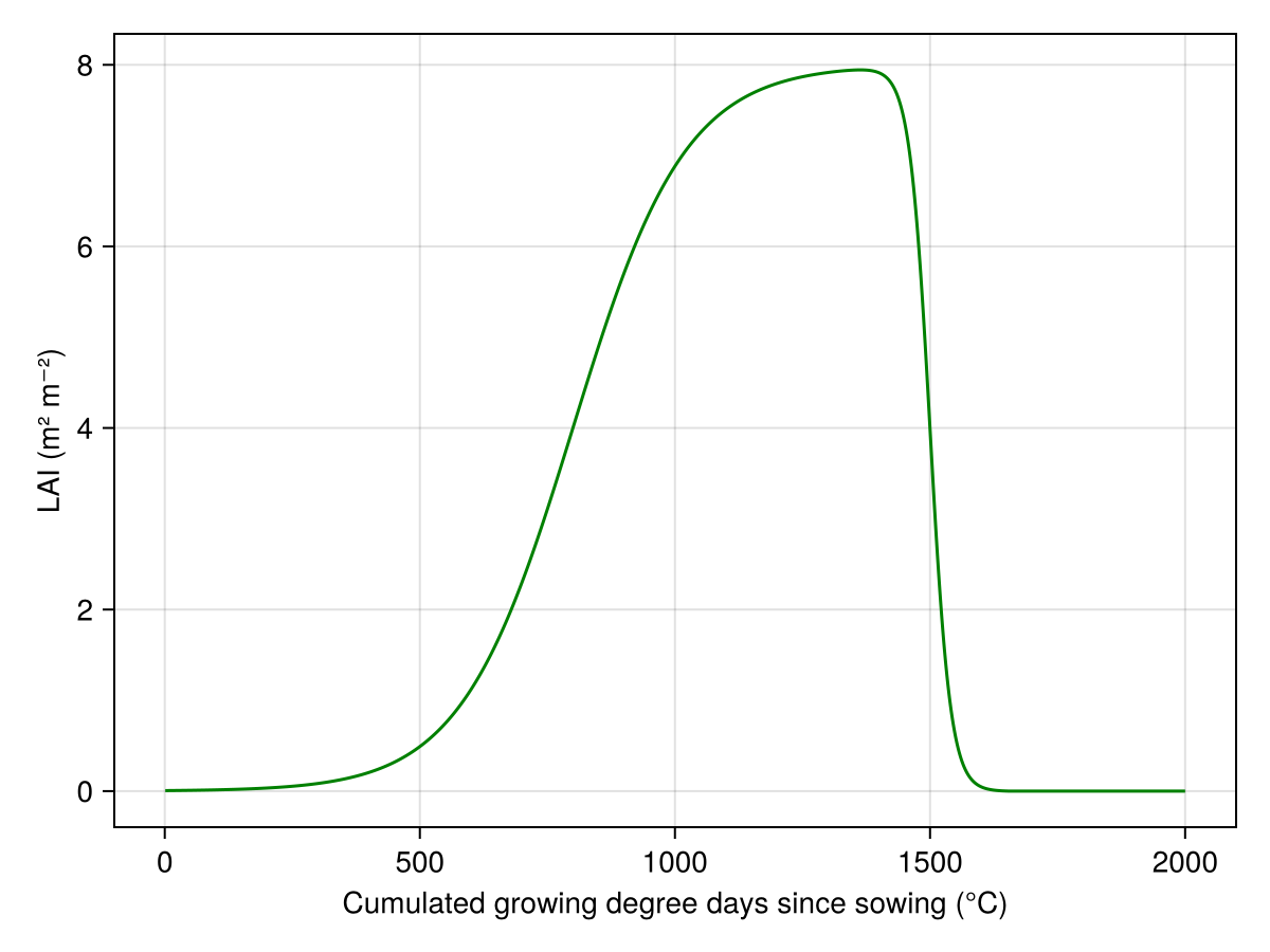
Model coupling
Model coupling is done automatically by the package, and is based on the dependency graph between the models. To couple models, we just have to add them to the ModelList. For example, let's couple the ToyLAIModel with a model for light interception based on Beer's law:
# ] add PlantSimEngine, DataFrames, CSV
using PlantSimEngine, PlantMeteo, DataFrames, CSV

# Import the examples defined in the `Examples` sub-module
using PlantSimEngine.Examples

# Import the example meteorological data:
meteo_day = CSV.read(joinpath(pkgdir(PlantSimEngine), "examples/meteo_day.csv"), DataFrame, header=18)

# Define the list of models for coupling:
model2 = ModelList(
    ToyLAIModel(),
    Beer(0.6),
    status=(TT_cu=cumsum(meteo_day[:, :TT]),),  # Pass the cumulated degree-days as input to `ToyLAIModel`, this could also be done using another model
)

# Run the simulation:
run!(model2, meteo_day)

status(model2)
TimeStepTable{Status{(:TT_cu, :LAI, :aPPFD)...}(365 x 3):
╭─────┬──────────┬────────────┬───────────╮
│ Row │ TT_cu │ LAI │ aPPFD │
│ │ Float64 │ Float64 │ Float64 │
├─────┼──────────┼────────────┼───────────┤
│ 1 │ 0.0 │ 0.00554988 │ 0.0476221 │
│ 2 │ 0.0 │ 0.00554988 │ 0.0260688 │
│ 3 │ 0.0 │ 0.00554988 │ 0.0377774 │
│ 4 │ 0.0 │ 0.00554988 │ 0.0468871 │
│ 5 │ 0.0 │ 0.00554988 │ 0.0545266 │
│ 6 │ 0.0 │ 0.00554988 │ 0.0567055 │
│ 7 │ 0.0 │ 0.00554988 │ 0.0521376 │
│ 8 │ 0.0 │ 0.00554988 │ 0.0563642 │
│ 9 │ 0.0 │ 0.00554988 │ 0.0349947 │
│ 10 │ 0.0 │ 0.00554988 │ 0.0168016 │
│ 11 │ 0.0 │ 0.00554988 │ 0.0606171 │
│ 12 │ 0.0 │ 0.00554988 │ 0.0486197 │
│ 13 │ 0.5625 │ 0.00557831 │ 0.0357278 │
│ 14 │ 0.945833 │ 0.00559777 │ 0.0519777 │
│ 15 │ 0.979167 │ 0.00559946 │ 0.0564167 │
│ ⋮ │ ⋮ │ ⋮ │ ⋮ │
╰─────┴──────────┴────────────┴───────────╯
350 rows omitted
The ModelList couples the models by automatically computing the dependency graph of the models. The resulting dependency graph is:
╭──── Dependency graph ──────────────────────────────────────────╮
│  ╭──── LAI_Dynamic ─────────────────────────────────────────╮  │
│  │  ╭──── Main model ────────╮                              │  │
│  │  │  Process: LAI_Dynamic  │                              │  │
│  │  │  Model: ToyLAIModel    │                              │  │
│  │  │  Dep: nothing          │                              │  │
│  │  ╰────────────────────────╯                              │  │
│  │                  │  ╭──── Soft-coupled model ─────────╮  │  │
│  │                  │  │  Process: light_interception    │  │  │
│  │                  └──│  Model: Beer                    │  │  │
│  │                     │  Dep: (LAI_Dynamic = (:LAI,),)  │  │  │
│  │                     ╰─────────────────────────────────╯  │  │
│  ╰──────────────────────────────────────────────────────────╯  │
╰────────────────────────────────────────────────────────────────╯
We can plot the results by indexing the model with the variable name (e.g. model2[:LAI]):
using CairoMakie

fig = Figure(resolution=(800, 600))
ax = Axis(fig[1, 1], ylabel="LAI (m² m⁻²)")
lines!(ax, model2[:TT_cu], model2[:LAI], color=:mediumseagreen)

ax2 = Axis(fig[2, 1], xlabel="Cumulated growing degree days since sowing (°C)", ylabel="aPPFD (mol m⁻² d⁻¹)")
lines!(ax2, model2[:TT_cu], model2[:aPPFD], color=:firebrick1)

fig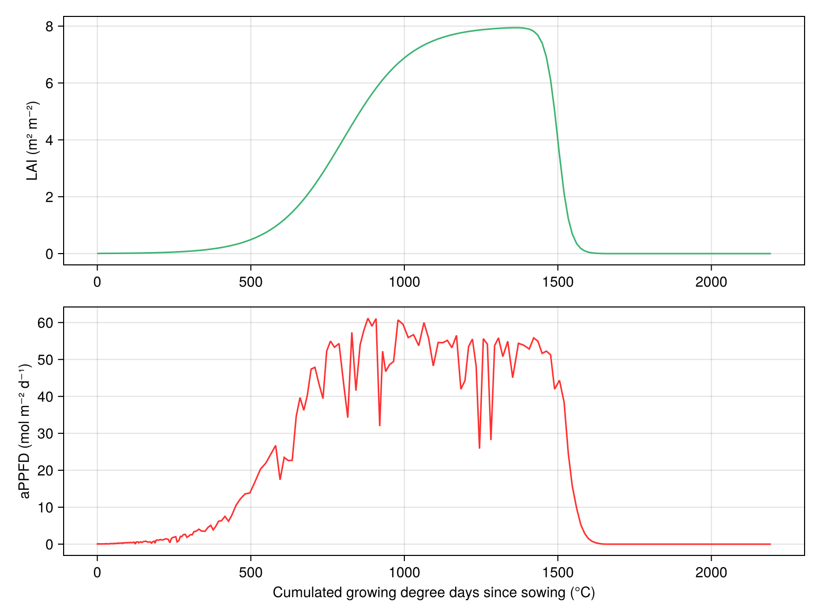
Multiscale modelling
See the Multi-scale modeling section for more details.
The package is designed to be easily scalable, and can be used to simulate models at different scales. For example, you can simulate a model at the leaf scale, and then couple it with models at any other scale, e.g. internode, plant, soil, scene scales. Here's an example of a simple model that simulates plant growth using sub-models operating at different scales:
mapping = Dict(
    "Scene" => ToyDegreeDaysCumulModel(),
    "Plant" => (
        MultiScaleModel(
            model=ToyLAIModel(),
            mapping=[
                :TT_cu => "Scene",
            ],
        ),
        Beer(0.6),
        MultiScaleModel(
            model=ToyAssimModel(),
            mapping=[:soil_water_content => "Soil"],
        ),
        MultiScaleModel(
            model=ToyCAllocationModel(),
            mapping=[
                :carbon_demand => ["Leaf", "Internode"],
                :carbon_allocation => ["Leaf", "Internode"]
            ],
        ),
        MultiScaleModel(
            model=ToyPlantRmModel(),
            mapping=[:Rm_organs => ["Leaf" => :Rm, "Internode" => :Rm],],
        ),
    ),
    "Internode" => (
        MultiScaleModel(
            model=ToyCDemandModel(optimal_biomass=10.0, development_duration=200.0),
            mapping=[:TT => "Scene",],
        ),
        MultiScaleModel(
            model=ToyInternodeEmergence(TT_emergence=20.0),
            mapping=[:TT_cu => "Scene"],
        ),
        ToyMaintenanceRespirationModel(1.5, 0.06, 25.0, 0.6, 0.004),
        Status(carbon_biomass=1.0)
    ),
    "Leaf" => (
        MultiScaleModel(
            model=ToyCDemandModel(optimal_biomass=10.0, development_duration=200.0),
            mapping=[:TT => "Scene",],
        ),
        ToyMaintenanceRespirationModel(2.1, 0.06, 25.0, 1.0, 0.025),
        Status(carbon_biomass=1.0)
    ),
    "Soil" => (
        ToySoilWaterModel(),
    ),
);
We can import an example plant from the package:
mtg = import_mtg_example()/ 1: Scene
├─ / 2: Soil
└─ + 3: Plant
└─ / 4: Internode
├─ + 5: Leaf
└─ < 6: Internode
└─ + 7: Leaf
Make a fake meteorological data:
meteo = Weather(
    [
    Atmosphere(T=20.0, Wind=1.0, Rh=0.65, Ri_PAR_f=300.0),
    Atmosphere(T=25.0, Wind=0.5, Rh=0.8, Ri_PAR_f=500.0)
]
);
And run the simulation:
out_vars = Dict(
    "Scene" => (:TT_cu,),
    "Plant" => (:carbon_allocation, :carbon_assimilation, :soil_water_content, :aPPFD, :TT_cu, :LAI),
    "Leaf" => (:carbon_demand, :carbon_allocation),
    "Internode" => (:carbon_demand, :carbon_allocation),
    "Soil" => (:soil_water_content,),
)

out = run!(mtg, mapping, meteo, outputs=out_vars, executor=SequentialEx());
We can then extract the outputs in a DataFrame and sort them:
using DataFrames
df_out = outputs(out, DataFrame)
sort!(df_out, [:timestep, :node])| Row | timestep | organ | node | carbon_allocation | TT_cu | carbon_assimilation | aPPFD | LAI | soil_water_content | carbon_demand |
|---|---|---|---|---|---|---|---|---|---|---|
| Int64 | String | Int64 | Union… | Union… | Union… | Union… | Union… | Union… | Union… | |
| 1 | 1 | Scene | 1 | 10.0 | ||||||
| 2 | 1 | Soil | 2 | 0.5 | ||||||
| 3 | 1 | Plant | 3 | 10.0 | 0.499037 | 4.99037 | 0.00607765 | 0.5 | ||
| 4 | 1 | Internode | 4 | 0.124183 | 0.5 | |||||
| 5 | 1 | Leaf | 5 | 0.124183 | 0.5 | |||||
| 6 | 1 | Internode | 6 | 0.124183 | 0.5 | |||||
| 7 | 1 | Leaf | 7 | 0.124183 | 0.5 | |||||
| 8 | 2 | Scene | 1 | 25.0 | ||||||
| 9 | 2 | Soil | 2 | 0.5 | ||||||
| 10 | 2 | Plant | 3 | 25.0 | 0.952884 | 9.52884 | 0.00696482 | 0.5 | ||
| 11 | 2 | Internode | 4 | 0.157992 | 0.75 | |||||
| 12 | 2 | Leaf | 5 | 0.157992 | 0.75 | |||||
| 13 | 2 | Internode | 6 | 0.157992 | 0.75 | |||||
| 14 | 2 | Leaf | 7 | 0.157992 | 0.75 | |||||
| 15 | 2 | Internode | 8 | 0.157992 | 0.75 | |||||
| 16 | 2 | Leaf | 9 | 0.157992 | 0.75 |
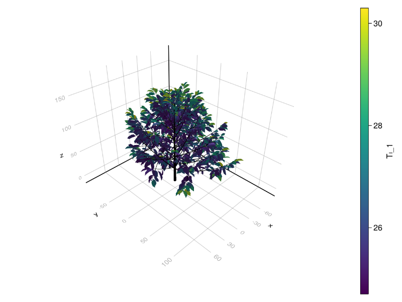
An example output of a multiscale simulation is shown in the documentation of PlantBiophysics.jl:
Projects that use PlantSimEngine
Take a look at these projects that use PlantSimEngine:
Make it yours
The package is developed so anyone can easily implement plant/crop models, use it freely and as you want thanks to its MIT license.
If you develop such tools and it is not on the list yet, please make a PR or contact me so we can add it! 😃